Estimation of the prevalence and incidence of motor neuron diseases in two Spanish regions: Catalonia and Valencia

Design

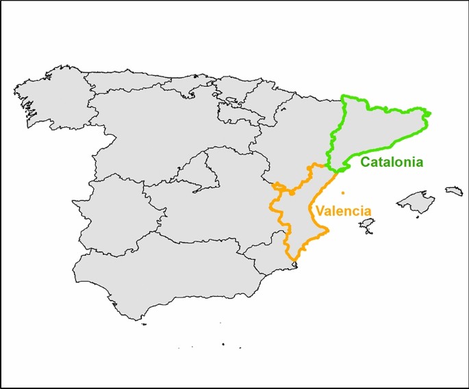
Two Spanish Mediterranean regions were analysed, Catalonia and Valencia, which together comprise 26.72% of the total Spanish population and 53.67% of the Spanish population living in the Mediterranean basin (Catalonia 7,566,000 inhabitants and Valencia 4,975,000 inhabitants)²⁵ (Fig. 1). These two neighbouring regions share climatic and sociodemographic conditions and have a common history (both belonged to the Kingdom of Aragon, one of the two kingdoms comprising Spain from the Middle Ages onwards), and much of the Catalan population originates from Valencia and vice-versa. Thus, it is likely that these populations have shared genetic and environmental risk factors of MND.

Location of the Catalonia and Valencia regions.

The study population was made up of the residents in the regions of Catalonia and Valencia between 1 January 2011 and 31 December 2019 (Catalonia) and between 1 January 2013 and 31 December 2018 (Valencia).

Two population-based cohorts were used, (one from Catalonia and the other from Valencia), encompassing the entire population of both regions. In both cohorts, clinical data were prospectively obtained, while some demographic data were retrospectively collected. The cohorts included all the patients who had been assessed at two Motor Neuron Disease Functional Units (MNDFU) in Spain: the Bellvitge University Hospital in Hospitalet de Llobregat in Catalonia, and the La Fe University and Polytechnic Hospital in Valencia, which act as referral units in the Catalan and Valencian regions, respectively. All the patients with MND seen in the Bellvitge Hospital since 2011 and the La Fe Hospital since 2013 were recorded prospectively in a database created for this purpose, and which included their demographic and clinical characteristics. All the patients studied were adults (specifically, the minimum age was 21 years in the Valencia cohort and 25 in the Catalonia cohort).

This study included the patients who had been evaluated in either of the two referral units during the time periods stated above and who met the following criteria: (1) a diagnosis of ALS, defined as the presence of UMN and LMN dysfunction in at least one body region at any time of the disease course, or LMN dysfunction in at least two body regions with a disease course typical of ALS (continuous non-invasive ventilation or death within four years from disease onset)²⁶; (2) a diagnosis of definite PLS according to recent criteria³; (3) PMA diagnosis, considered as the presence of isolated signs of LMN in at least two body regions with a slowly progressing disease course and a prolonged survival (> 4 years). Although there is no agreed consensus about the definition of PMA, to be consistent with the definition used for PLS, the recently proposed four-year criteria from Al-Chalabi et al.¹ was used. The diagnosis of MND and its different diagnostic categories (ALS, PLS and PMA) was made by specialists in MND.

All the census tracts of all the municipalities in Catalonia and Valencia were included; some with cases of MND and others (a much higher number) with no cases.

Variables

Response variable

Different models were estimated depending on the response variable. First, all MND cases were considered as the response variable, regardless of diagnostic category. Second, the following diagnostic categories were considered as additional response variables: ALS, PLS and. PMA. This was done separately for each region (Catalonia and Valencia).

Individual control variables

Age at diagnosis and sex were included as individual explanatory variables. Age was further categorised into quintiles, taking the first quintile as the reference category. For the sex variable, male was considered as the reference category.

Patients were further categorized, according to the symptom of onset, into spinal, bulbar, respiratory and cognitive. The C9ORF72 expansion was studied in all MND patients, whereas SOD1 was sequenced in those familial MND patients not carrying the C9ORF72 expansion. In PMA patients, expansions in the androgen receptor gene were appropriately excluded.

Contextual control variables

The Spanish Epidemiology Association’s Deprivation Index 2011 (IP2011)²⁷ corresponding to each of the census tracts of the municipalities of each of the two regions, was included as a contextual explanatory variable of interest. The IP2011 combines the information on six socioeconomic indicators, calculated for each census tract and based on the data collected in the Spanish Population and Housing Census 2011²⁸: percentage of the manual worker population, percentage of the temporary working population, percentage of the unemployed population, percentage of the population without complete compulsory schooling, and percentage of primary residences without access to the Internet The IP2011 was considered as the first component of a sequential principal component analysis (PCA). First, a PCA with ten selected indicators was carried out (in addition to the six already mentioned, the following were included: the percentage of the population born in low-income countries and arrived in Spain after 2006, the percentage of the population born in low-income countries or born in Spain whose father or mother were born in low-income countries, the percentage of the population aged 65 or over, and the percentage of single-parent households with a woman in charge). Second, the ten indicators were correlated (using Spearman’s correlation coefficient) with the first component obtained through the PCA. Third, those indicators with correlations less than 0.5 were excluded. Finally, a PCA was carried out using the six indicators finally considered (further information can be found in²⁷). The deprivation index was categorised into quintiles, taking the first quintile (i.e. the one corresponding to the less economically deprived census tracts) as the reference category.

The populations in each of the two regions, stratified by sex and age groups (women under 16 years, women aged 16 to 64 years, women ≥ 65 years, men under 16 years, men aged 16 to 64 years, men ≥ 65 years), were also included as contextual explanatory variables. The reference categories were the youngest categories for each sex. The total population at risk (population aged over 16 years) was used as the offset in the model for each of the two regions.

Population data by census tract, age, and sex was obtained from the Spanish Population and Housing Census 2011²⁸.

The graphic representation was produced based on the cartography of Catalonia (SRC ED50/UTM zone 31 N) and Valencia (SRC ED50/UTM zone 30 N) at the census tract level for 2011²⁹.

Statistical analysis

Selection bias is common in observational designs. That is, the analysed cohorts do not constitute a random sample of the population. Some subjects have a higher probability of being observed than others and, therefore, of being present in the sample. To this effect, the subjects that come into contact with one of the referral MNDFUs in the regions studied will be overrepresented.

If the selection was exogenous (also termed ignorable non-response, missing at random, or selection on observables), or in other words if the probability of a subject to be observed was identical for all subjects, weighting the sample to give less weight to the subjects actually observed would be sufficient. The weighting used would be the same as the inverse of the percentage of subjects among the population seen at each hospital, stratified by sex and age group. In epidemiology, this method of weighting is called standardisation by age and sex³⁰, considering the population covered by each hospital as the standard population.

However, these subjects are very likely to go to one of the referral MNDFUs, not only because they have symptoms of the onset of the disease, but also because there are unobserved factors that influence their use, which would be correlated with the non-observable factors that affect the response variable³¹. In this sense, the population served by the MNDFU has a centre bias. In other words, they do not serve all the patients in the respective populations, but rather a part that may be biased (e.g. some centres send more patients than others; the patients they send are younger than the real population, etc.). In all cases, the probability of these subjects being observed is not the same for all the subjects. Therefore, weighting (standardisation) by age and sex would not correct the selection bias³¹.

In this case (known as endogenous selection, also termed informative selection, missing not at random, or selection on unobservables), other more complex statistical methods should be used to obtain unbiased estimates of prevalence and incidence, something that standardization by age and sex does not permit. Therefore, we chose a two-part model³². In the first part, the probability of a subject being observed is estimated. These probabilities are then used as weightings in the second part of the model, where the prevalence and incidence are estimated, with the aim of correcting the non-randomness (in other words, the selection bias). The two parts are typically estimated using a two-part model called Hurdle^32,33. Thus, we specified a Hurdle model in which the two components were estimated jointly³³.

In the first part, the probability that an individual is being observed is modelled using a generalised linear mixed model (GLMM) with a binomial link. Included as variables associated with this probability are those that could explain that a subject was observed (in other words, that he/she had had contact with the UFMN of the corresponding hospital). More specifically, we considered individual and contextual variables.

Conditional on the true risk at the location \({x}_{i}\), the probability of a case (of the corresponding response variable) occurring in this location, \(P\left({x}_{i}\right)\), \(i=1,\dots , n\), is distributed as a binomial.

\({n.trials}_{i}\) is the population at risk of being a case in the location \({x}_{i}\).

The link function is as follows:

where the subindex \(i\) indicates the census tract of the municipalities in each of the two regions and \(\beta\) are the coefficients of the explanatory variables (\({e}^{\beta }\) is the relative risk associated with each of them). \(\eta\) and \(S\) are random effects. \(\eta\) indicates the spatially unstructured individual heterogeneity. In other words, it indicates the non-observable confounders associated with every individual which do not vary over time. \(S\) is a spatially structured random effect normally distributed with zero mean and a Mátérn covariance function:

where \({\mathrm{\rm K}}_{\nu }\) is the modified Bessel function of the second type and order \(\nu >0\). \(\nu\) is a smoother parameter, \({\sigma }^{2}\) is the variance and \(\kappa >0\) is related to the range (\(\rho =\sqrt{8 \nu }/\kappa\)), the distance to which the spatial correlation is close to 0.1.

Because of the large number of census tracts with no cases, in the second part a GLMM with Zero Inflated Poisson distribution is used to model the number of patients diagnosed for each of the response variables and by census tract. The same explanatory variables as in the first part of the model are included.

Conditional to the true risk in the location \({x}_{i}\), the mathematic expectation of cases of the response variable occurring in each of the census tracts, \(\theta \left({x}_{i}\right)\), \(i=1,\dots , n\), is distributed as a Poisson:

In this case, the link function is as follows:

The definition of the parameters, the variables, and the random effects, is the same as described previously.

In both parts, random effects that include non-observed confounders are also included, capturing individual heterogeneity (specific for each of the two parts) and spatial dependence. That is to say, areas that are close in space show more similar prevalence and incidence than areas that are not close (common to the two parts). In the model used to estimate the incidence, an additional random effect was included to control for the existence of temporal trends (also common to the two parts). The temporal dependence was controlled using a random effect structured as a random walk of order 1³⁴ (further details can be found elsewhere³³).

Both parts were estimated simultaneously following a Bayesian perspective, using the Integrated Nested Laplace Approximation (INLA) approach³⁵. Priors that penalize the complexity (PC priors)³⁶ and have been found to be very robust were used.

Consequently, point and interval estimates were obtained for the prevalence and the incidence, both at the level of the region to which the hospital belongs, and at the level of census tract of each of their municipalities.

Last, the prevalence and incidence of MND per 100,000 inhabitants is represented on the map of the census tracts of Catalonia and Valencia using the mapping by census tracts of the Population and Housing Census 2011²⁸, and the “leaflet” library³⁷ (Figs. 3 and 4).

All analyses were carried out using the free software R (version 3.6.2)³⁸, through the INLA package^35,39.

Ethics approval

The data for this study came from an anonymised clinical administrative database and only the lead researcher, where necessary, had access to the identity of each individual. The information in this administrative clinical database was obtained through the informed consent of the patients. In any case, all methods of this study were carried out in accordance with relevant guidelines and regulations, having been revised and approved by the Committee of Ethics and Clinical Research (CEIC) of the Bellvitge University Hospital.